I don’t get as excited about American Community Survey data releases as I used to. My primary interest is the commute mode share data, and at least in Madison that just doesn’t change much year to year. But hey, you can never be sure and so when the data is out, I have to quickly run my analysis.
Madison
No surprises: Madison commute share didn’t change between 2024 and 2025 in a statistically significant way.
Show code
library(tidycensus)
library(tidyverse)
library(gt)


get_msn_mode_share <- function(year, state = "WI", city = "Madison city, Wisconsin") {
  acs_data <- get_acs(year = year, survey = "acs1", table = "S0801", geography = "place", state = state, cache_table=T)
  acs_data |>
    filter(NAME == city) |>
    mutate(year = year)
}


mode_share <- map_dfr(c(2010:2019, 2021:2025), get_msn_mode_share)

mode_share <- mode_share |>
  mutate(gender = case_when(str_detect(variable, "^S0801_C01") ~ "total",
                            str_detect(variable, "^S0801_C02") ~ "male",
                            str_detect(variable, "^S0801_C03") ~ "female"),
         mode_readable = case_when(
           str_detect(variable, "S0801_C0[1-3]_002") ~ "Drive",
           str_detect(variable, "S0801_C0[1-3]_009") ~ "Transit",
           str_detect(variable, "S0801_C0[1-3]_010") ~ "Walk",
           str_detect(variable, "S0801_C0[1-3]_011") ~ "Bike",
           str_detect(variable, "S0801_C0[1-3]_013") ~ "Work from home"))

# data frame for the ggrepel labels on the right of the plot
mode_share_2025 <-  mode_share |>
  filter(year == 2025 & !is.na(mode_readable))


mode_share |>
  filter(!is.na(mode_readable) & gender == "total" & year >= 2024) |>
  group_by(mode_readable, year) |>
  pivot_wider(names_from = year, values_from = c(estimate, moe)) |>
  mutate(change = estimate_2025 - estimate_2024,
         sig_diff = significance(estimate_2024, estimate_2025, moe_2024, moe_2025),
         sig_diff = if_else(sig_diff == TRUE, "yes", "-")) |>
  select(mode_readable, estimate_2024,  moe_2024, estimate_2025, moe_2025, change, sig_diff) |>
  ungroup() |>
  gt() |>
  tab_header(title = "Change in commute mode share in Madison, WI") |>
  fmt_percent(columns = c(estimate_2024,
                          estimate_2025,
                          moe_2024,
                          moe_2025), decimals = 1, scale_values = F) |>
  fmt_percent(columns = c(change), decimals = 1, scale_values = F, force_sign = T) |>
  tab_spanner(label = "2024",
              columns = c(estimate_2024, moe_2024)) |>
  tab_spanner(label = "2025",
              columns = ends_with("_2025")) |>
  tab_spanner(
    label = "Mode share",
    columns = c(estimate_2024,
                moe_2024,
                estimate_2025,
                moe_2025)
  ) |>
  cols_label(mode_readable = "Commute mode",
             estimate_2024 = "Estimate",
             moe_2024 = "+/-",
             estimate_2025 = "Estimate",
             moe_2025 = "+/-",
             change = "Change (percentage points)",
             sig_diff = "statistically significant?") |>
  data_color(
    columns = c(change),
    colors = scales::col_numeric(
      palette = "viridis",
      domain = NULL )) |>
  tab_source_note(
    source_note = "Data: American Community Survey 1-year estimates, Table S0801. Visualization: Harald Kliems"
)| Change in commute mode share in Madison, WI | ||||||
|
Mode share
|
||||||
|---|---|---|---|---|---|---|
| Commute mode |
2024
|
2025
|
Change (percentage points) | statistically significant? | ||
| Estimate | +/- | Estimate | +/- | |||
| Drive | 64.3% | 2.2% | 65.4% | 2.8% | +1.1% | - |
| Transit | 7.6% | 1.1% | 7.1% | 1.2% | −0.5% | - |
| Walk | 6.6% | 1.2% | 6.9% | 1.7% | +0.3% | - |
| Bike | 3.4% | 0.8% | 3.7% | 1.3% | +0.3% | - |
| Work from home | 16.8% | 1.7% | 15.6% | 1.7% | −1.2% | - |
| Data: American Community Survey 1-year estimates, Table S0801. Visualization: Harald Kliems | ||||||
They city’s first Bus Rapid Transit route opened in late 2024. One could have reasonably expected that to drive up the transit commute share, but it doesn’t show. Will we see the impact of high gas prices in next year’s data? I’m rather skeptical. While a lot of people are complaining about them, I’m not sure it is going to lead to much behavioral impact on commute trips.
Zooming out, we see that commuting by car is still below pre-pandemic rates and working from home is way up.
Show code
mode_share |>
  filter(!is.na(mode_readable) & gender == "total") |>
  group_by(mode_readable, year) |>
  ggplot(aes(year, estimate, color = mode_readable)) +
  geom_line(linewidth = 1.2) +
  hrbrthemes::scale_color_ipsum(
    #name = element_blank()
  ) +
  geom_pointrange(aes(ymin = estimate - moe, ymax = estimate + moe), alpha = .8,
                  size = 1,fatten = 1) +
  hrbrthemes::theme_ipsum_rc() +
  scale_x_continuous(breaks = c(2010, 2015, 2019, 2023, 2025), minor_breaks = NULL, limits = c(2010, 2026.5)) +
  ylab("estimate (%)") +
  labs(title = "Mode share stabilized after the pandemic disruption",
       subtitle ="Madison (WI) commute mode share, 2010-2025",
       caption = "American Community Survey 1-year estimates, Table S0801\nVisualization: Harald Kliems") +
  theme(legend.position = "none") +
ggrepel::geom_text_repel(data = mode_share_2025 |> filter(gender == "total"), aes(label = paste0(mode_readable, " ", estimate, "%")), nudge_x = 1) 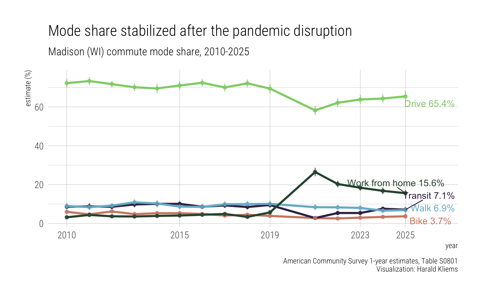
Milwaukee
What about Wisconsin’s largest city, Milwaukee? Here we can actually see statistically significant changes in driving and biking.
Show code
mode_share <- map_dfr(c(2010:2019, 2021:2025), ~ get_msn_mode_share (.x, city = "Milwaukee city, Wisconsin"))

mode_share <- mode_share |>
  mutate(gender = case_when(str_detect(variable, "^S0801_C01") ~ "total",
                            str_detect(variable, "^S0801_C02") ~ "male",
                            str_detect(variable, "^S0801_C03") ~ "female"),
         mode_readable = case_when(
           str_detect(variable, "S0801_C0[1-3]_002") ~ "Drive",
           str_detect(variable, "S0801_C0[1-3]_009") ~ "Transit",
           str_detect(variable, "S0801_C0[1-3]_010") ~ "Walk",
           str_detect(variable, "S0801_C0[1-3]_011") ~ "Bike",
           str_detect(variable, "S0801_C0[1-3]_013") ~ "Work from home"))

# data frame for the ggrepel labels on the right of the plot
mode_share_2025 <-  mode_share |>
  filter(year == 2025 & !is.na(mode_readable))


mode_share |>
  filter(!is.na(mode_readable) & gender == "total" & year >= 2024) |>
  group_by(mode_readable, year) |>
  pivot_wider(names_from = year, values_from = c(estimate, moe)) |>
  mutate(change = estimate_2025 - estimate_2024,
         sig_diff = significance(estimate_2024, estimate_2025, moe_2024, moe_2025),
         sig_diff = if_else(sig_diff == TRUE, "yes", "-")) |>
  select(mode_readable, estimate_2024,  moe_2024, estimate_2025, moe_2025, change, sig_diff) |>
  ungroup() |>
  gt() |>
  tab_header(title = "Change in commute mode share in Milwaukee, WI") |>
  fmt_percent(columns = c(estimate_2024,
                          estimate_2025,
                          moe_2024,
                          moe_2025), decimals = 1, scale_values = F) |>
  fmt_percent(columns = c(change), decimals = 1, scale_values = F, force_sign = T) |>
  tab_spanner(label = "2024",
              columns = c(estimate_2024, moe_2024)) |>
  tab_spanner(label = "2025",
              columns = ends_with("_2025")) |>
  tab_spanner(
    label = "Mode share",
    columns = c(estimate_2024,
                moe_2024,
                estimate_2025,
                moe_2025)
  ) |>
  cols_label(mode_readable = "Commute mode",
             estimate_2024 = "Estimate",
             moe_2024 = "+/-",
             estimate_2025 = "Estimate",
             moe_2025 = "+/-",
             change = "Change (percentage points)",
             sig_diff = "statistically significant?") |>
  data_color(
    columns = c(change),
    colors = scales::col_numeric(
      palette = "viridis",
      domain = NULL )) |>
  tab_source_note(
    source_note = "Data: American Community Survey 1-year estimates, Table S0801. Visualization: Harald Kliems"
)| Change in commute mode share in Milwaukee, WI | ||||||
|
Mode share
|
||||||
|---|---|---|---|---|---|---|
| Commute mode |
2024
|
2025
|
Change (percentage points) | statistically significant? | ||
| Estimate | +/- | Estimate | +/- | |||
| Drive | 75.8% | 1.5% | 78.0% | 1.6% | +2.2% | yes |
| Transit | 5.4% | 0.8% | 5.2% | 1.1% | −0.2% | - |
| Walk | 4.9% | 1.0% | 4.2% | 0.6% | −0.7% | - |
| Bike | 0.7% | 0.3% | 0.3% | 0.1% | −0.4% | yes |
| Work from home | 10.9% | 1.2% | 10.6% | 1.5% | −0.3% | - |
| Data: American Community Survey 1-year estimates, Table S0801. Visualization: Harald Kliems | ||||||
Driving is up slightly and bike commuting down a lot (from an already low starting point). I don’t have any explanations to offer.
Cambridge, MA
Since an online mutual from Cambridge posted about the data on Bluesky, I quickly created the table for this low drive mode share city.
Show code
mode_share <- map_dfr(c(2010:2019, 2021:2025), ~ get_msn_mode_share (.x, city = "Cambridge city, Massachusetts", state = "MA"))

mode_share <- mode_share |>
  mutate(gender = case_when(str_detect(variable, "^S0801_C01") ~ "total",
                            str_detect(variable, "^S0801_C02") ~ "male",
                            str_detect(variable, "^S0801_C03") ~ "female"),
         mode_readable = case_when(
           str_detect(variable, "S0801_C0[1-3]_002") ~ "Drive",
           str_detect(variable, "S0801_C0[1-3]_009") ~ "Transit",
           str_detect(variable, "S0801_C0[1-3]_010") ~ "Walk",
           str_detect(variable, "S0801_C0[1-3]_011") ~ "Bike",
           str_detect(variable, "S0801_C0[1-3]_013") ~ "Work from home"))

# data frame for the ggrepel labels on the right of the plot
mode_share_2025 <-  mode_share |>
  filter(year == 2025 & !is.na(mode_readable))


mode_share |>
  filter(!is.na(mode_readable) & gender == "total" & year >= 2024) |>
  group_by(mode_readable, year) |>
  pivot_wider(names_from = year, values_from = c(estimate, moe)) |>
  mutate(change = estimate_2025 - estimate_2024,
         sig_diff = significance(estimate_2024, estimate_2025, moe_2024, moe_2025),
         sig_diff = if_else(sig_diff == TRUE, "yes", "-")) |>
  select(mode_readable, estimate_2024,  moe_2024, estimate_2025, moe_2025, change, sig_diff) |>
  ungroup() |>
  gt() |>
  tab_header(title = "Change in commute mode share in Cambridge, MA") |>
  fmt_percent(columns = c(estimate_2024,
                          estimate_2025,
                          moe_2024,
                          moe_2025), decimals = 1, scale_values = F) |>
  fmt_percent(columns = c(change), decimals = 1, scale_values = F, force_sign = T) |>
  tab_spanner(label = "2024",
              columns = c(estimate_2024, moe_2024)) |>
  tab_spanner(label = "2025",
              columns = ends_with("_2025")) |>
  tab_spanner(
    label = "Mode share",
    columns = c(estimate_2024,
                moe_2024,
                estimate_2025,
                moe_2025)
  ) |>
  cols_label(mode_readable = "Commute mode",
             estimate_2024 = "Estimate",
             moe_2024 = "+/-",
             estimate_2025 = "Estimate",
             moe_2025 = "+/-",
             change = "Change (percentage points)",
             sig_diff = "statistically significant?") |>
  data_color(
    columns = c(change),
    colors = scales::col_numeric(
      palette = "viridis",
      domain = NULL )) |>
  tab_source_note(
    source_note = "Data: American Community Survey 1-year estimates, Table S0801. Visualization: Harald Kliems"
)| Change in commute mode share in Cambridge, MA | ||||||
|
Mode share
|
||||||
|---|---|---|---|---|---|---|
| Commute mode |
2024
|
2025
|
Change (percentage points) | statistically significant? | ||
| Estimate | +/- | Estimate | +/- | |||
| Drive | 25.2% | 3.0% | 23.9% | 3.4% | −1.3% | - |
| Transit | 19.2% | 2.5% | 25.9% | 3.0% | +6.7% | yes |
| Walk | 21.5% | 2.9% | 22.5% | 2.8% | +1.0% | - |
| Bike | 11.4% | 2.6% | 9.4% | 2.3% | −2.0% | - |
| Work from home | 20.1% | 2.7% | 17.0% | 2.9% | −3.1% | - |
| Data: American Community Survey 1-year estimates, Table S0801. Visualization: Harald Kliems | ||||||
Transit is up a lot, which my mutual attributes to improvements to the MBTA’s Red Line.
You can use the above code to generate tables and charts for your city. Just replace the city and state in this code chunk.
Or shoot me an email with your city.