Sometimes you get sucked into a data rabbit hole. For reasons I don’t exactly remember, I got interested in households with a lot of cars. Here’s a quick blog post about households with 4 or more vehicles available, based on data from the American Community Survey. We limit the analysis to the 100 cities with the largest population (my preferred way of doing it because it includes the city I live in, Madison, Wisconsin).
Let’s start with a map:
Show code
get_pop <- function(state) {
  get_acs("place", table = "B01003", state = state, cache_table = TRUE)
}

pop <- map_dfr(datasets::state.abb, get_pop)

pop_100_states <- pop |>
  arrange(desc(estimate)) |>
  head(100) |>
  mutate(state = str_sub(GEOID, start = 0, end = 2)) |>
  distinct(state)

pop_100_cities <- pop |>
  arrange(desc(estimate)) |>
  head(100) |>
  pull(NAME)


get_cars <- function(state) {
  get_acs("place",
    table = "B08201",
    summary_var = "B08201_001",
    state = state, cache_table = TRUE, geometry = T
  )
}

cars <- map_dfr(pop_100_states, get_cars)

tmap_mode("view")
cars |>
  filter(NAME %in% pop_100_cities) |>
  filter(variable == "B08201_006") |>
  mutate(
    cars_4_pct = estimate / summary_est,
    cars_4_pct_label = scales::percent(cars_4_pct)
  ) |>
  arrange(desc(cars_4_pct)) |>
  tm_shape() +
  tm_dots(
    title = "4+-car households",
    col = "cars_4_pct",
    id = "NAME",
    popup.vars = c("Share of 4+-car households" = "cars_4_pct_label"),
    legend.format = list(fun = function(x) paste0(formatC(x * 100, digits = 0, format = "f"), " %")),
    style = "jenks"
  ) +
  tm_layout(title = "High-car ownership in US cities") +
  tm_credits("100 largest US cities. Data: American Community Survey")
Some patterns appear to emerge, but let’s look at the top and bottom ten of the list in a table:
Show code
top_bottom_vector <- c(top_bottom = rep("Highest %", 10), rep("Lowest %", 10))

top_bottom <- cars |>
  sf::st_drop_geometry() |>
  filter(NAME %in% pop_100_cities) |>
  filter(variable == "B08201_006") |>
  mutate(
    cars_4_pct = estimate / summary_est,
    NAME = str_remove(NAME, " city")
  ) |>
  arrange(desc(cars_4_pct))

top <- head(top_bottom, 10) |> mutate(top_bottom = "Highest %")
bottom <- tail(top_bottom, 10) |> mutate(top_bottom = "Lowest %")

top_bottom_table <- rbind(top, bottom)

top_bottom_table |>
  group_by(top_bottom) |>
  select(NAME, estimate, cars_4_pct, top_bottom) |>
  gt() |>
  tab_header(
    title = "US cities with the highest and lowest % of owning 4+ cars",
    subtitle = "100 most populous cities"
  ) |>
  fmt_percent(columns = cars_4_pct, decimals = 1) |>
  fmt_number(estimate, use_seps = TRUE, decimals = 0) |>
  tab_spanner("4+ car households", columns = c(estimate, cars_4_pct)) |>
  cols_label(NAME = "City", estimate = "number", cars_4_pct = "percent") |>
  tab_source_note("American Community Survey, 5-year estimates, 2017-2021. Table B08201") |>
  opt_table_font(stack = "industrial") |>
  tab_style(
    style = cell_text(weight = "bold"),
    locations = cells_row_groups()
)| US cities with the highest and lowest % of owning 4+ cars | ||
| 100 most populous cities | ||
| City | 4+ car households | |
|---|---|---|
| number | percent | |
| Highest % | ||
| Santa Ana, California | 12,754 | 16.6% |
| Riverside, California | 11,683 | 13.2% |
| Chula Vista, California | 10,656 | 12.9% |
| Anaheim, California | 12,730 | 12.3% |
| San Jose, California | 36,761 | 11.3% |
| Santa Clarita, California | 8,182 | 11.2% |
| Stockton, California | 9,785 | 10.2% |
| Garland, Texas | 7,881 | 9.9% |
| Laredo, Texas | 7,142 | 9.8% |
| Fremont, California | 6,791 | 9.1% |
| Lowest % | ||
| Atlanta, Georgia | 4,467 | 2.0% |
| St. Louis, Missouri | 2,621 | 1.9% |
| Baltimore, Maryland | 4,474 | 1.8% |
| Pittsburgh, Pennsylvania | 2,151 | 1.6% |
| Buffalo, New York | 1,789 | 1.5% |
| Philadelphia, Pennsylvania | 9,067 | 1.4% |
| Boston, Massachusetts | 3,431 | 1.3% |
| Newark, New Jersey | 1,370 | 1.2% |
| Jersey City, New Jersey | 1,026 | 0.9% |
| New York, New York | 26,323 | 0.8% |
| American Community Survey, 5-year estimates, 2017-2021. Table B08201 | ||
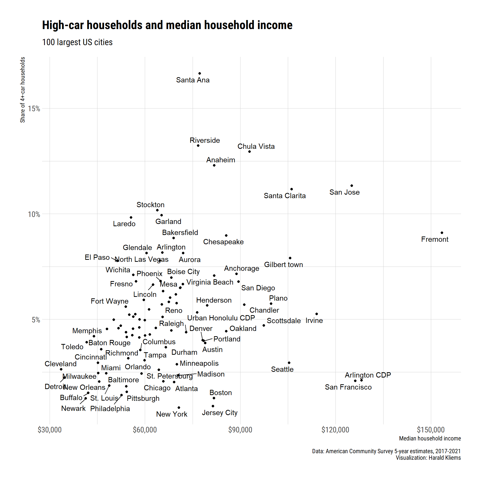
What can explain the difference? Is it something uniquely Californian and Texan that has people owning so many cars? One thing to look is median household income. Places with higher incomes probably afford more car ownership.
Show code
get_income <- function(state) {
  get_acs("place",
    table = "B19013", survey = "acs5",
    state = state, cache_table = TRUE, geometry = FALSE
  )
}

income <- map_dfr(pop_100_states, get_income)

income |>
  filter(NAME %in% pop_100_cities) |>
  left_join(top_bottom, by = "GEOID") |>
  mutate(
    short_name = str_extract(NAME.x, "^([^,]*)"),
    short_name = str_remove(short_name, " city| municipality"),
    median_income = estimate.x
  ) |>
  ggplot(aes(median_income, cars_4_pct, label = short_name)) +
  ggrepel::geom_text_repel() +
  geom_point() +
  scale_x_continuous(name = "Median household income", labels = scales::label_dollar()) +
  scale_y_continuous(name = "Share of 4+-car households", labels = scales::label_percent()) +
  theme_ipsum_rc() +
  labs(
    title = "High-car households and median household income",
    subtitle = "100 largest US cities",
    caption = "Data: American Community Survey 5-year estimates, 2017-2021\nVisualization: Harald Kliems"
  )
We should also look at the average household size. Maybe cities with a high share of 4+-car households just have larger households!
Show code
get_hh_size <- function(state) {
  get_acs("place",
    variable = "B25010_001", survey = "acs5",
    state = state, cache_table = TRUE, geometry = FALSE
  )
}


hh_size <- map_dfr(pop_100_states, get_hh_size)

hh_size |>
  filter(NAME %in% pop_100_cities) |>
  left_join(top_bottom, by = "GEOID") |>
  mutate(
    short_name = str_extract(NAME.x, "^([^,]*)"),
    short_name = str_remove(short_name, " city| municipality"),
    hh_size = estimate.x
  ) |>
  ggplot(aes(hh_size, cars_4_pct, label = short_name)) +
  ggrepel::geom_text_repel() +
  geom_point() +
  scale_x_continuous(name = "Mean household size") +
  scale_y_continuous(name = "Share of 4+-car households", labels = scales::label_percent()) +
  theme_ipsum_rc() +
  labs(
    title = "High-car households and average household size",
    subtitle = "100 largest US cities",
    caption = "Data: American Community Survey 5-year estimates, 2017-2021\nVisualization: Harald Kliems"
  )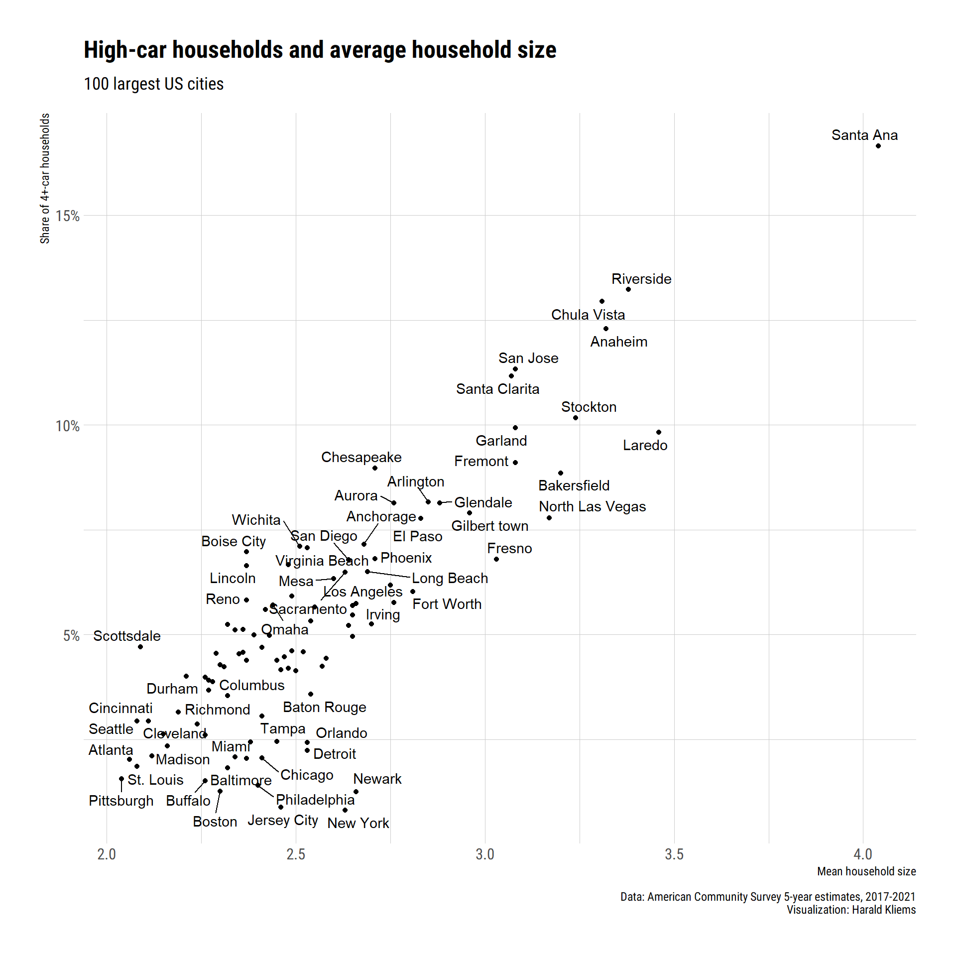
And yes, there’s a very strong relationship! Of course there are outliers such as New York and Boston—which probably tell us we should add an indicator for cities with a good public transit system. While it’s not perfect, we use transit commute mode share as our variable.
Show code
get_transit <- function(state) {
  get_acs("place",
    table = "S0801", survey = "acs5",
    state = state, cache_table = TRUE, geometry = FALSE
  )
}


transit <- map_dfr(pop_100_states, get_transit)

transit |>
  filter(NAME %in% pop_100_cities) |>
  filter(variable == "S0801_C01_009") |>
  left_join(top_bottom, by = "GEOID") |>
  mutate(
    short_name = str_extract(NAME.x, "^([^,]*)"),
    short_name = str_remove(short_name, " city| municipality"),
    transit_share = estimate.x
  ) |>
  ggplot(aes(transit_share, cars_4_pct, label = short_name)) +
  ggrepel::geom_text_repel() +
  geom_point() +
  # scale_x_continuous(name = "Median household income", labels = scales::label_dollar()) +
  scale_y_continuous(name = "Share of 4+-car households", labels = scales::label_percent()) +
  theme_ipsum_rc() +
  labs(
    title = "High-car households and transit commuting mode share",
    subtitle = "100 largest US cities",
    caption = "Data: American Community Survey 5-year estimates, 2017-2021\nVisualization: Harald Kliems"
)![]()
High transit cities have few high-car households; but within low transit cities, there’s still a lot of variability.
If this weren’t just a quick post, I’d probably try building a model that takes income, household size, and transit mode share together. But I’ll leave that for another day or someone else.
Bonus table (revised: 2024-03-02)
After publishing this article, I received feedback. Given the chart about household sizes, it would be interesting to look at the number of vehicles by household size. That makes sense: There’s a difference between a one-person household having 4+ cars and a four-person household doing so. The data is available, and we can calculate the percentage of households that have more cars than people in it. Here’s the new top/bottom ten table:
Show code
over_car_vars <- c(10, 11, 12, 17, 18, 24)

filter_vars <- map_chr(over_car_vars, function(x) {
  paste0("B08201_0", x)
})


over_cars <- cars |>
  sf::st_drop_geometry() |>
  filter(NAME %in% pop_100_cities) |>
  pivot_wider(id_cols = c(GEOID, NAME), names_from = "variable", values_from = "estimate") |>
  rowwise() |>
  mutate(over_car = sum(!!!syms(filter_vars)) / B08201_001)


top_bottom <- over_cars |> arrange(desc(over_car))

top <- head(top_bottom, 10) |> mutate(top_bottom = "Highest %")
bottom <- tail(top_bottom, 10) |> mutate(top_bottom = "Lowest %")

top_bottom_table <- rbind(top, bottom)

top_bottom_table |>
  group_by(top_bottom) |>
  select(NAME, over_car, top_bottom) |>
  mutate(NAME = str_remove(NAME, " city| municipality")) |>
  gt() |>
  tab_header(
    title = "US cities with the highest and lowest % households with more cars than people",
    subtitle = "100 most populous cities"
  ) |>
  fmt_percent(columns = over_car, decimals = 1) |>
  cols_label(NAME = "City", over_car = "percentage of households") |>
  tab_source_note("American Community Survey, 5-year estimates, 2017-2021. Table B08201") |>
  opt_table_font(stack = "industrial") |>
  tab_style(
    style = cell_text(weight = "bold"),
    locations = cells_row_groups()
)| US cities with the highest and lowest % households with more cars than people | |
| 100 most populous cities | |
| City | percentage of households |
|---|---|
| Highest % | |
| Chesapeake, Virginia | 15.6% |
| Boise City, Idaho | 14.6% |
| Virginia Beach, Virginia | 13.8% |
| Anchorage, Alaska | 12.9% |
| Wichita, Kansas | 12.6% |
| Colorado Springs, Colorado | 12.6% |
| Winston-Salem, North Carolina | 12.5% |
| Spokane, Washington | 12.0% |
| Oklahoma City, Oklahoma | 11.7% |
| Albuquerque, New Mexico | 11.5% |
| Lowest % | |
| Baltimore, Maryland | 4.5% |
| Buffalo, New York | 4.5% |
| Miami, Florida | 3.3% |
| San Francisco, California | 3.2% |
| Chicago, Illinois | 3.1% |
| Philadelphia, Pennsylvania | 3.0% |
| Newark, New Jersey | 2.5% |
| Boston, Massachusetts | 2.1% |
| Jersey City, New Jersey | 1.1% |
| New York, New York | 1.0% |
| American Community Survey, 5-year estimates, 2017-2021. Table B08201 | |