The Journal Sentinel recently ran an article on population growth (or the lack thereof) yesterday. Conveniently, that day’s #30DayMapChallenge also happened to be “population,” and the JS article didn’t include any maps. So let’s create a map of the population change figures.
The data
Population estimates are produced by the Wisconsin Department of Administration, and they compare current estimates with the 2020 decennial census numbers. The WSJ article uses the “Municipality Final Population Estimates, Alphabetical List” file, and so will we.
Show code
Rows: 1,861
Columns: 11
$ doa_code                 <chr> "10201", "43002", "34002", "01201",…
$ fips_5                   <chr> "00100", "00175", "00225", "00275",…
$ muni_type                <chr> "C", "T", "T", "C", "T", "T", "T", …
$ municipality_name        <chr> "Abbotsford", "Abrams", "Ackley", "…
$ county                   <chr> "In Multiple Counties", "Oconto", "…
$ final_estimate_2023      <dbl> 2375, 2000, 465, 1736, 1379, 543, 1…
$ census_2020              <dbl> 2275, 1960, 467, 1761, 1378, 540, 1…
$ numeric_change           <dbl> 100, 40, -2, -25, 1, 3, 19, -42, -6…
$ percent_change           <dbl> 0.0440, 0.0204, -0.0043, -0.0142, 0…
$ voting_age_estimate_2023 <dbl> 1746, 1579, 385, 1380, 1154, 433, 1…
$ voting_age_census_2020   <dbl> 1665, 1541, 385, 1394, 1148, 429, 1…
The article excludes cities with fewer than 30,000 residents. Setting thresholds is always a balancing act, but a threshold of 30,000 residents is quite high. For example, Verona or Middleton, both sizable suburbs of Madison, continue to see large population growth, but their total populations are only about 15,000 and 23,000, respectively. So let’s set a threshold of 15,000 for now and see how it goes.
Note that the municipality_name variable has some strange numbers after some names. If we look back at the spreadsheet, those are footnotes. This will cause problems when joining the growth data with geographic datasets, and so we’ll either have to clean those names or use the fips_5 variable instead. We will do the latter, as that may also help avoid issues caused by duplicate names or differences in spelling.
Next we need geographic data. As per usual, the tigris package should be easiest.
Rows: 806
Columns: 13
$ STATEFP    <chr> "55", "55", "55", "55", "55", "55", "55", "55", "…
$ PLACEFP    <chr> "01000", "33275", "34825", "37225", "71975", "480…
$ PLACENS    <chr> "01582672", "01583366", "01583393", "01583435", "…
$ AFFGEOID   <chr> "1600000US5501000", "1600000US5533275", "1600000U…
$ GEOID      <chr> "5501000", "5533275", "5534825", "5537225", "5571…
$ NAME       <chr> "Algoma", "Hawkins", "Hillsboro", "Ironton", "Sca…
$ NAMELSAD   <chr> "Algoma city", "Hawkins village", "Hillsboro city…
$ STUSPS     <chr> "WI", "WI", "WI", "WI", "WI", "WI", "WI", "WI", "…
$ STATE_NAME <chr> "Wisconsin", "Wisconsin", "Wisconsin", "Wisconsin…
$ LSAD       <chr> "25", "47", "25", "47", "47", "25", "25", "25", "…
$ ALAND      <dbl> 6362282, 5712401, 3638454, 862597, 2262888, 20609…
$ AWATER     <dbl> 114522, 48938, 98551, 3866, 347671, 55411136, 542…
$ geometry   <MULTIPOLYGON [°]> MULTIPOLYGON (((-87.46487 4..., MULT…
Let’s do a join.
Show code
growth_sf <- wi_places %>%
  inner_join(growth, by = join_by(PLACEFP == fips_5))
Looks good! Now we can start mapping, starting with something simple
Show code
# get Wisconsin county map
wi_counties <- counties(state = "WI", cb = TRUE)

tm_shape(wi_counties) +
  tm_polygons() +
  tm_shape(growth_sf) +
  tm_bubbles(col = "percent_change", size = "percent_change", style = "jenks") +
  tm_text("NAME", auto.placement = TRUE, size = .5) +
  tmap::tm_layout(legend.outside = TRUE)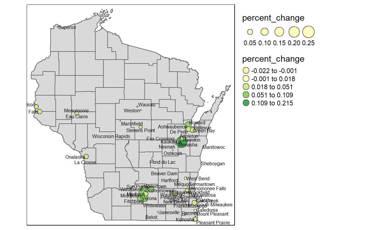
That’s a good start, but there are too many cities, the breaks don’t quite work and the labeling needs work. I spent a good amount of time trying out different options, but I’ll rest-of-the-f’ing-owl that process. Here’s a decent looking panel of two maps, one for the fastest growing and one for shrinking Wisconsin municipalities.
Show code
shrunk_lg_growth <- growth_sf |>
  filter(percent_change >= 0.04 | percent_change < -0.01) |>
  mutate(abs_percent_change = abs(percent_change),
         shrink_grow = if_else(percent_change < 0, "shrink", "grow"),
         name_label = paste0(NAME, " ", scales::label_percent(accuracy = 0.1)(percent_change)))

bbox_new <- st_bbox(wi_counties) # current bounding box

xrange <- bbox_new$xmax - bbox_new$xmin # range of x values
yrange <- bbox_new$ymax - bbox_new$ymin # range of y values

  bbox_new[1] <- bbox_new[1] - (0.1 * xrange) # xmin - left
 bbox_new[3] <- bbox_new[3] + (0.1 * xrange) # xmax - right
 bbox_new[2] <- bbox_new[2] - (0.02 * yrange) # ymin - bottom
 # bbox_new[4] <- bbox_new[4] + (0.5 * yrange) # ymax - top

bbox_new <- bbox_new %>%  # take the bounding box ...
  st_as_sfc() # ... and make it a sf polygon


tm_shape(wi_counties, bbox = bbox_new ) +
    tm_polygons()+
  tm_shape(shrunk_lg_growth) +
  tm_bubbles(col = "shrink_grow", size = "abs_percent_change") +
  tm_text("name_label",
          size = .7,
          auto.placement = TRUE) +
  tmap::tm_layout(legend.show = FALSE,
    legend.outside = TRUE,
                  legend.outside.position = "bottom",
                  panel.labels = c("Municipalities with > 4% growth", "Municipalities that lost > 1% population"))  +
    tm_facets(by = "shrink_grow", ncol = 1)
As you can see, the included municipalities differ from the ones highlighted in the article. This is because of the different population and growth/shrinkage cut-offs. And yet, the overall conclusion of the article can be seen in these maps as well: “A shrinking population in Milwaukee, and other large cities, has been counterbalanced by a growing population in Madison, which is one of the few areas in the state to experience such an increase since 2020.”