Map fun with City of Madison tax parcel data

Building age, property use, and architectural styles in Madison

The City of Madison’s open data portal has a tax parcel dataset. Tax information, however, is not the only thing included in the dataset. There are over 140 variables and for this post we will look at three of them: The year the structure on the parcel was built, the use of the property, and the architectural style.

Correction 2023-02-21: The originally published version of this post used the BuiltYear variable for the map of the age of buildings. Jim Kreft pointed out that there is another variable in the dataset, Maxconstru, which has more complete data. The code and map have been updated accordingly.

Show code

library(sf)
library(tidyverse)


buildings <- read_sf("/Users/user1/Downloads/Tax_Parcels_(Assessor_Property_Information)/Tax_Parcels_(Assessor_Property_Information).shp")
buildings <- buildings |> 
  st_make_valid()

Building age

Let’s start with the YearBuilt variable. This allows us a glimpse into the development of Madison over time. First, a static map:

Show code

buildings2 <- buildings |> 
  mutate(MaxConstru = na_if(MaxConstru, 0),
         MaxConstru_labels = cut(MaxConstru,
                                breaks = c(-Inf, 1900, 1945, 1980, 2000, 2010, Inf),
                                labels = c("pre-1900", "1900 to 1944", "post-WWII to 1979", "1980 to 1999", "2000 to 2009", "2010 and newer"),
                                ordered_result = T))

library(tmap)
tmap_mode("plot")
tmap_options(bg.color = "black", legend.text.color = "white")
p <- buildings2 |> 
  select(MaxConstru_labels) |> 
  tm_shape() +
  tm_polygons(title = "", "MaxConstru_labels", border.alpha = 0, style = "cont",
              colorNA = "darkgrey") +
  tm_credits("Map: @HaraldKliems. Data: City of Madison Tax Parcels", col = "white") +
  tm_layout(title = "How old are Madison’s buildings?",
            scale = 1,
            bg.color = "black",
            legend.text.color = "white",
            title.color = "white",
            legend.title.color = "white")

# tmap_save(p, filename = "c:/Users/user1/Desktop/map.png", width = 12, height = 9, dpi = 600)
p

It’d be nice to have an interactive map, but the dataset is too large to not crash most browsers (stay tuned; I’m working on alternatives).

In the static map it’s not easy to see areas where parcels have redeveloped, such as along the East Washington Ave corridor, but we can make out some glimpses. We also see that a lot of parcels have missing data, and that missingness doesn’t seem to be random. It’d be interesting to know why the city has better data on some properties/areas/eras than on others!

Property use

The age of a structure only tells us part of a story. How is a building use, and how do these uses cluster? The property use data has many different categories, and to keep the map legible we need to lump a lot of them together. This is what we get for the 10 most common uses:

Show code

p2 <- buildings2 |>
  select(PropertyUs) |>
  mutate(PropertyUs = case_when(
    str_detect(PropertyUs, "Apartment$") ~ "Apartment",
    str_detect(PropertyUs, "^Condominium") ~ "Condominium",
    TRUE ~ PropertyUs
  )) |>
  mutate(PropertyUs_collapsed = fct_lump_n(PropertyUs, 10)) |>
  tm_shape() +
  tm_polygons(
    title = "",
    "PropertyUs_collapsed",
    border.alpha = 0,
    colorNA = "ghostwhite"
  ) +
  tm_credits("Map: @HaraldKliems. Data: City of Madison Tax Parcels") +
  tm_layout(
    title = "Property use for tax parcels in Madison",
    scale = .6,
    bg.color = "black",
    legend.text.color = "white",
    title.color = "white",
    legend.title.color = "white"
  )

tmap_mode("plot")
p2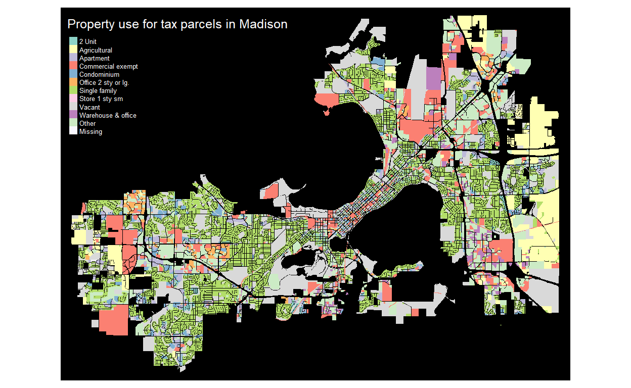

Home style

A third and final map looks at the “home style.”

Show code

p3 <- buildings2 |>
  select(HomeStyle) |>
  mutate(
    HomeStyle = case_when(
      str_detect(HomeStyle, "^Ranch") ~ "Ranch",
      str_detect(HomeStyle, "^Townhouse") ~ "Townhouse",
      str_detect(HomeStyle, "^Garden") ~ "Garden",
      TRUE ~ HomeStyle
    ),
    HomeStyle_collapsed = fct_lump_n(HomeStyle, 10)
  ) |>
  tm_shape() +
  tm_polygons("HomeStyle_collapsed",
              border.alpha = 0,
              colorNA = "ghostwhite") +
  tm_credits("Map: @HaraldKliems. Data: City of Madison Tax Parcels") +
  tm_layout(
    title = "Architectural style of Madison buildings",
    scale = .6,
    bg.color = "black",
    legend.text.color = "white",
    title.color = "white",
    legend.title.color = "white"
  )

tmap_mode("plot")
p3

Lumping together the less common styles under “Other” is a little unfortunate for this variable. It’ll make use miss out on less common but interesting architectural styles such as “Spanish mediterranean” or “New style modern international”. So let’s at least have a table with all the styles and how common they are.

Show code

buildings2 |> st_drop_geometry() |>
  select(HomeStyle) |>
  mutate(HomeStyle = case_when(str_detect(HomeStyle, "^Ranch") ~ "Ranch",
                               str_detect(HomeStyle, "^Townhouse") ~ "Townhouse",
                               str_detect(HomeStyle, "^Garden") ~ "Garden",
                               TRUE ~ HomeStyle)) |>
           group_by(HomeStyle) |>
           tally(sort = T) |>
  DT::datatable()